
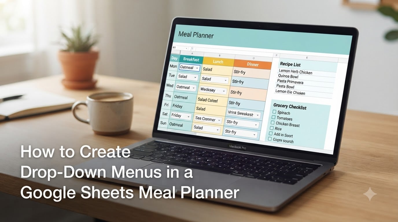
If you have ever spent ten minutes typing out the same breakfast options across seven rows of a spreadsheet, you already know why drop-down menus are a game-changer for meal planning. I built my first Google Sheets meal planner back in 2023, and adding dropdowns cut my weekly planning time from twenty minutes to about three. The trick is a built-in Google Sheets feature called data validation, which lets you turn any cell into a selectable list of options.
Yes, you can absolutely create a dropdown menu in Google Sheets without any add-ons or coding. The feature works on both desktop and mobile, and once you set it up, clicking a cell reveals a clean list of meal options you pick from instead of typing. This guide walks through the entire process from scratch, covering everything from your first basic dropdown to advanced tricks like dependent dropdowns and auto-populating grocery lists.
By the end, you will have a fully functional meal planner with dropdown menus for every meal slot, a recipe database that feeds those dropdowns, and a shopping list that builds itself based on what you selected. Let us start with the foundation.
Table of Contents
- What Drop-Down Menus Are and Why They Matter in a Meal Planner
- Setting Up Your Google Sheets Meal Planner Structure
- How to Access Data Validation in Google Sheets
- Step-by-Step: Creating Your First Dropdown Menu
- Creating Dropdowns from a Range vs Predefined Values
- Building a Recipe Dropdown List for Your Meal Plan
- Organizing Weekly Meals with Day-of-Week Dropdowns
- Advanced Dropdown Options: Colors, Chips, and Multi-Select
- Creating Dependent Dropdowns for Meal Type Filters
- Auto-Populating a Grocery List from Your Dropdown Selections
- How to Copy and Reuse Dropdowns Across Your Sheet
- Using Dropdowns on the Google Sheets Mobile App
- Troubleshooting Common Dropdown Issues
- Frequently Asked Questions
- Can you create a dropdown menu in Google Sheets?
- How do I create a dropdown menu in the Google Sheets app?
- How do I create a dynamic drop-down list in Google Sheets?
- How do I turn a column into a Dropdown list in Google Sheets?
- Does Google Sheets have a meal planner?
- How to build a planner in Google Sheets?
- How do I create a dropdown list for data validation in Google Sheets?
- Final Thoughts on Building Your Meal Planner Dropdowns
What Drop-Down Menus Are and Why They Matter in a Meal Planner
A drop-down menu in Google Sheets is an in-cell selection tool created through data validation that restricts input to a list of predefined choices. When you click a cell with a dropdown applied, a small arrow appears and you pick from the available options instead of typing freely. For meal planning, this means every breakfast, lunch, dinner, and snack cell becomes a one-click selector from your personal recipe list.
The benefits go beyond convenience. Dropdowns enforce consistency across your sheet, which matters when you are building automated grocery lists or tracking nutrition data. If one cell says “Spaghetti Bolognese” and another says “spagetti bolognese,” formulas will not match them. A dropdown eliminates that problem entirely because every selection comes from a controlled vocabulary.
I have tested meal planners with and without dropdowns, and the difference is significant. A plain-text meal planner takes about three times longer to fill out and is far more prone to typos. A dropdown-equipped planner feels closer to using a dedicated meal planning app, except it lives in a spreadsheet you fully control.
Setting Up Your Google Sheets Meal Planner Structure
Before building any dropdowns, you need a clean sheet layout. The most requested structure in spreadsheet communities is the 3-tab system: one tab for your weekly calendar, one for your recipe database, and one for your shopping list. I use this exact setup and it works beautifully.
Create three tabs at the bottom of your Google Sheet by clicking the plus icon. Name the first tab “Meal Plan,” the second “Recipes,” and the third “Shopping List.” This separation keeps your data organized and makes dropdown creation much easier, because each dropdown will pull options from the Recipes tab.
On the Recipes tab, set up columns for Recipe Name, Category (Breakfast, Lunch, Dinner, Snack), and Ingredients. List every meal you cook regularly, one per row. This list becomes the source data for your dropdown menus on the Meal Plan tab. A solid starter list might include 15 to 20 recipes across all categories.
On the Meal Plan tab, create a grid with days of the week as rows and meal types as columns. Your column headers should be Breakfast, Lunch, Dinner, and Snack. The cells where days and meals intersect are exactly where your dropdown menus will go. This is the layout users on Reddit repeatedly ask about, and it maps perfectly to how people think about their weekly food schedule.
How to Access Data Validation in Google Sheets
Data validation lives under the Data menu in Google Sheets. Click any cell (or select a range of cells), then navigate to Data > Data validation in the top menu bar. A sidebar opens on the right side of your screen where you configure the dropdown settings. This is the control panel for every dropdown you create.
If you do not see “Data validation” immediately, look for “Data validation rules” in the dropdown. Google occasionally renames menu items, but the function is always under the Data menu. The keyboard shortcut is not available for this, so menu navigation is your path in.
The data validation sidebar shows a button labeled “Add Rule.” Click it to start creating a new dropdown. From here, Google Sheets gives you two main paths: dropdown from a list of items you type in manually, or dropdown from a range of cells in your sheet. Both approaches have specific use cases in meal planning.
Step-by-Step: Creating Your First Dropdown Menu
Here is the exact process for creating your first dropdown using predefined values. I will use a Breakfast column as the example.
Step 1: Select the cells where you want the dropdown. On your Meal Plan tab, click and drag to highlight all seven cells under the Breakfast column (one for each day of the week).
Step 2: Go to Data > Data validation in the top menu. The sidebar opens on the right.
Step 3: Click “Add Rule.” Google Sheets presents criteria options. The top choice is “Dropdown,” which is what you want.
Step 4: In the options section, you will see default entries like “Option 1” and “Option 2.” Click each one and replace the text with your actual meal options. For breakfast, type entries like “Oatmeal,” “Scrambled Eggs,” “Smoothie,” and “Yogurt Parfait.”
Step 5: Each option has a color dot next to it. Click the dot to assign a color to each meal. This gives you instant visual distinction when scanning your weekly plan.
Step 6: Scroll down to advanced options if needed. You can set what happens when someone types a value that is not in the list: either reject the input or show a warning. For a personal meal planner, “Show warning” works fine. For a shared planner, “Reject input” prevents messy data.
Step 7: Click “Done.” Your selected cells now have dropdown arrows. Click any cell to see your breakfast options pop up as a clean list. Pick one and it fills the cell with your chosen color.
Creating Dropdowns from a Range vs Predefined Values
Google Sheets offers two ways to populate a dropdown, and understanding the difference saves you hours of maintenance. The choice between them depends on how often your meal list changes.
Dropdown (predefined values): You type the options directly into the data validation sidebar. This is fast for short, stable lists like meal types (Breakfast, Lunch, Dinner) or day names (Monday through Sunday). The downside is that adding a new option requires opening data validation and editing the rule manually.
Dropdown (from range): The dropdown pulls its options from a range of cells elsewhere in your sheet. If you point it at the Recipe Name column on your Recipes tab, every recipe you add to that column automatically appears in the dropdown. No editing the rule needed. This is the better choice for recipe lists, because you will constantly add new meals to your rotation.
Here is the decision rule I use: if the list has fewer than 8 items and rarely changes, use predefined values. If the list grows over time or you want to add items without touching validation rules, use a range. For a meal planner, your recipe dropdowns should always use ranges.
To create a dropdown from a range, follow the same steps as above, but in Step 4 choose “Dropdown (from range)” instead of “Dropdown.” A field appears where you type or select the cell range. For your recipe list, select the entire Recipe Name column on the Recipes tab, something like Recipes!A2:A100. Using a generous range like A2:A100 means any new recipe you add up to row 100 automatically shows in the dropdown.
Building a Recipe Dropdown List for Your Meal Plan
Now let us build the actual recipe dropdown that powers your meal planner. This is where the two tabs start working together.
First, make sure your Recipes tab is populated. You need at least a handful of meals listed in column A with headers in row 1. Each row below the header is one recipe. For a functional starter system, aim for at least 10 recipes across breakfast, lunch, and dinner categories.
Go to your Meal Plan tab and select all the cells under the Dinner column (seven cells for seven days). Open Data > Data validation and click “Add Rule.” Choose “Dropdown (from range)” and then click the grid icon in the range field. Navigate to your Recipes tab and select the range covering your dinner recipe names, for example Recipes!A2:A50. Click OK and then Done.
Now every dinner cell on your Meal Plan tab has a dropdown showing all your dinner recipes. Click a cell, scroll through the list, and tap a recipe name. It fills in instantly with the color formatting you configured.
Here is the best part: when you add a new dinner recipe to row 51 on your Recipes tab, it automatically appears in every dinner dropdown on your Meal Plan tab. No rebuilding, no updating rules. This is the dynamic behavior that forum users constantly ask about, and the range-based approach handles it natively.
Repeat this process for your Lunch and Snack columns, pointing each one at the appropriate section of your Recipes tab. If your recipes are categorized in column B, you can filter the range or create separate sections on the Recipes tab for each meal type.
Organizing Weekly Meals with Day-of-Week Dropdowns
Some planners use a flexible layout where you select the day of the week itself from a dropdown, rather than having fixed day labels. This works well if your schedule varies or you want to plan around specific days dynamically.
Create a column called “Day” on your Meal Plan tab. Select the cells in that column and open data validation. Choose “Dropdown” (predefined values) and enter the seven days: Monday, Tuesday, Wednesday, Thursday, Friday, Saturday, and Sunday. Assign a unique color to each day for visual scanning.
This approach lets you drag rows around without losing the day association. You could also add special day labels like “Meal Prep Sunday” or “Leftover Wednesday” to match how you actually cook. The dropdown ensures spelling stays consistent, which matters if any formula references the day name.
I use a hybrid approach: fixed day labels in the row headers and a separate “Theme” dropdown column for meal themes like “Quick,” “Batch Cook,” or “Try Something New.” This gives structure while keeping flexibility for weeks when I want to experiment.
Advanced Dropdown Options: Colors, Chips, and Multi-Select
Google Sheets updated its dropdown feature to include display style options that affect how selections look in the cell. When creating or editing a dropdown rule, scroll to the “Display Style” section to choose between chips and arrows.
Chip style shows each selection as a pill-shaped colored chip inside the cell. This is the default for new dropdowns and works great for meal planners because the color makes it easy to spot patterns at a glance. A week of dinner chips in different colors tells you instantly whether you are eating too much of the same thing.
Arrow style shows a plain text value with a small arrow indicator on the right side of the cell. This is subtler and works better if your meal planner is shared in a professional or clinical setting where you want a cleaner look.
Color coding deserves special attention for meal planning. Assign green to vegetable-heavy meals, orange to comfort food, blue to quick-prep meals, and red to high-effort recipes. At a glance, your week becomes a color map that helps you balance effort and nutrition. I discovered this trick by accident and it completely changed how I plan.
Multiple selections are not natively supported by standard Google Sheets dropdowns. Each cell holds one selection at a time. If you need multiple values in one cell (for example, listing two side dishes), you have two workarounds. First, create separate columns for each side dish. Second, use Google Apps Script to build a custom multi-select function. The separate columns approach is simpler and works for most people.
Creating Dependent Dropdowns for Meal Type Filters
Dependent dropdowns are dropdowns whose options change based on what you selected in another cell. In meal planning, this means selecting “Breakfast” in one cell makes the next cell show only breakfast recipes. This is one of the most requested features in spreadsheet communities, and it is achievable with a combination of named ranges and the INDIRECT formula.
Here is how to set it up. First, organize your Recipes tab so each meal category has its own column: column A for Breakfast recipes, column B for Lunch, column C for Dinner. Select each column range and create a named range via Data > Named ranges. Name them “Breakfast,” “Lunch,” and “Dinner” respectively.
On your Meal Plan tab, create a “Meal Type” dropdown with three options: Breakfast, Lunch, Dinner. In the next cell over, create a “Dropdown (from range)” but instead of typing a fixed range, use the INDIRECT formula: INDIRECT(E2) where E2 is the cell containing your Meal Type selection. When you pick “Breakfast” in E2, the INDIRECT formula resolves to the named range called Breakfast, and the dropdown shows only breakfast recipes.
Change the meal type to “Lunch” and the same dropdown cell instantly shows only lunch options. This is the dependent dropdown behavior users want. It takes about ten minutes to set up but saves enormous time in daily use because you never scroll through irrelevant meal types.
One limitation: the INDIRECT formula reads the text in the meal type cell and matches it to a named range. The names must match exactly. If your meal type cell says “Breakfast,” your named range must be called “Breakfast” with identical spelling and capitalization. Test each meal type right after setup to confirm the linkage works.
Auto-Populating a Grocery List from Your Dropdown Selections
This is the feature that transforms a simple meal planner into something that feels automated. The goal is to have your Shopping List tab update itself based on what meals you selected on the Meal Plan tab. No manual list building.
The approach uses the VLOOKUP formula. On your Recipes tab, make sure column A is Recipe Name and column B lists the main ingredients. When you select “Chicken Stir-Fry” on your Meal Plan tab, the shopping list looks up that recipe, grabs the ingredients, and displays them.
On your Shopping List tab, set up a formula in cell A2 that references the first meal slot on your Meal Plan tab. Something like =VLOOKUP('Meal Plan'!B2, Recipes!A:B, 2, FALSE). This formula looks at what you selected in the Monday Breakfast cell (B2), searches for it in column A of the Recipes tab, and returns the matching ingredient list from column B.
Copy that formula down for every meal slot in your week. Now your shopping list tab shows the ingredients for every meal you planned, pulled automatically from your recipe database. Change a meal selection on the Meal Plan tab and the corresponding shopping list entry updates instantly.
For a cleaner list, wrap the formula in IFERROR to avoid showing errors on empty cells: =IFERROR(VLOOKUP('Meal Plan'!B2, Recipes!A:B, 2, FALSE), ""). This shows a blank cell instead of an error if no meal is selected yet.
If your ingredient lists are in a more detailed format (one ingredient per row instead of a comma-separated string in a single cell), you can use the FILTER or QUERY function instead of VLOOKUP to pull multiple rows. This advanced approach creates a true ingredient-level shopping list that aggregates duplicates across meals. For example, if three recipes use onions, the list shows “3x Onion” instead of three separate entries.
How to Copy and Reuse Dropdowns Across Your Sheet
Once you build a dropdown for one column, you do not need to rebuild it for similar columns. Google Sheets lets you copy validation rules between cells efficiently.
The simplest method is copy and paste. Select a cell that already has a dropdown, copy it with Ctrl+C (Cmd+C on Mac), then select the target cells and paste with Ctrl+V. The dropdown rule comes along with the paste. If you only want the validation rule without the cell content, use Edit > Paste special > Data validation only. This applies the rule while leaving existing cell content untouched.
For maintaining consistency across large sheets, named ranges are your best tool. If you create a named range called “AllRecipes” pointing to your recipe column, you can reference it by name in any dropdown. If you later expand the range (adding more recipes), you update the named range definition in one place and every dropdown using that name updates automatically.
I maintain a template sheet with dropdowns pre-configured for a generic week. When I want a fresh planning week, I duplicate the sheet and all dropdowns carry over. This is faster than rebuilding from scratch and ensures every week uses the same structure.
Using Dropdowns on the Google Sheets Mobile App
Creating dropdowns on mobile is more limited than on desktop, but it is possible for basic setups. The Google Sheets mobile app for iOS and Android supports viewing and selecting from existing dropdowns, though creating new ones requires a slightly different path.
To create a dropdown on mobile, open your sheet in the Google Sheets app and tap the cell where you want the dropdown. Tap the three-dot menu in the top right and select “Data validation.” From here, the interface mirrors the desktop version but with touch-optimized controls. You can add dropdown options, set colors, and choose between predefined values and range-based dropdowns.
The mobile app does not support named ranges creation, so if you need dependent dropdowns with INDIRECT, set those up on desktop first. Once configured, they work fine on mobile. Selecting from a dependent dropdown on your phone behaves exactly like on desktop.
Selecting from a dropdown on mobile works the same as desktop: tap the cell and choose from the list. The main difference is that you cannot multi-select cells on mobile, so applying a dropdown to a range of seven cells means selecting each one individually or doing the range selection through a different gesture (long-press and drag).
If your meal planner lives on a shared drive and other family members use it on their phones, test the mobile experience before relying on it. Some older versions of the Sheets app had rendering issues with chip-style dropdowns, though the current 2026 versions handle them well.
Troubleshooting Common Dropdown Issues
Even with perfect setup, dropdowns occasionally misbehave. Here are the most common problems and their fixes.
The dropdown arrow is not showing: This usually means the data validation rule was deleted or the cell formatting was overwritten. Click the cell, open Data validation, and check if a rule exists. If not, re-add it. If the rule exists but the arrow is hidden, the display style might be set to plain text instead of arrow or chip. Edit the rule and change the display style.
The dropdown shows old or missing options: If you are using a range-based dropdown, check that the range covers the new rows you added. A range set to Recipes!A2:A20 will not show recipes in row 21 and beyond. Expand the range to Recipes!A2:A100 or use an open-ended range. Named ranges solve this permanently because you can redefine them to cover more rows.
A warning appears when typing a valid meal name: This happens when the validation rule is set to “Reject input” and the typed text does not exactly match a dropdown option. Check for trailing spaces, different capitalization, or extra characters. The safest fix is to always select from the dropdown rather than typing, but if users insist on typing, switch the rule to “Show warning” instead of “Reject.”
The INDIRECT-dependent dropdown shows an error: This means the text in the trigger cell does not match any named range. Verify that the named range exists and that its name matches the dropdown value character-for-character. Named ranges are case-sensitive in Google Sheets, so “Breakfast” and “breakfast” are treated as different names.
Dropdowns disappeared after copying a sheet: When duplicating a sheet within the same workbook, validation rules should copy automatically. If they do not, the issue is usually that the copy references ranges on the original sheet rather than the new sheet. Check the range references in your validation rules after copying and update them to point to the correct sheet.
Frequently Asked Questions
Can you create a dropdown menu in Google Sheets?
Yes. Google Sheets has a built-in dropdown feature accessible through Data u0026gt; Data validation. You can create dropdowns from predefined values you type in or from a range of cells elsewhere in your sheet.
How do I create a dropdown menu in the Google Sheets app?
Open your sheet in the mobile app, tap the target cell, tap the three-dot menu, and select Data validation. You can add dropdown options with colors and choose between predefined values or range-based dropdowns, though named ranges must be set up on desktop first.
How do I create a dynamic drop-down list in Google Sheets?
Use a range-based dropdown pointing at a column of cells. Any new value added to that column automatically appears in the dropdown. For dependent dropdowns that change based on another selection, combine named ranges with the INDIRECT formula in the range field.
How do I turn a column into a Dropdown list in Google Sheets?
Select the entire column by clicking the column letter, then go to Data u0026gt; Data validation and click Add Rule. Choose Dropdown (from range), select the source range, and click Done. Every cell in the column now has a dropdown.
Does Google Sheets have a meal planner?
Google Sheets does not include a built-in meal planner template, but you can easily create one using dropdown menus for meal selection, a recipe database tab, and a grocery list tab. Many free community templates are also available that use dropdowns for meal planning.
How to build a planner in Google Sheets?
Create three tabs: Meal Plan, Recipes, and Shopping List. Populate the Recipes tab with your meals, add dropdown menus to the Meal Plan tab using Data validation set to Dropdown (from range), then use VLOOKUP formulas on the Shopping List tab to auto-populate ingredients based on your meal selections.
How do I create a dropdown list for data validation in Google Sheets?
Select your target cells, go to Data u0026gt; Data validation, click Add Rule, and choose Dropdown as the criteria. Type your options directly for short lists, or select a cell range to pull options dynamically from elsewhere in your sheet.
Final Thoughts on Building Your Meal Planner Dropdowns
Creating drop-down menus in a Google Sheets meal planner comes down to three core skills: data validation for the dropdowns themselves, range references for dynamic recipe lists, and formulas like VLOOKUP and INDIRECT for connecting your tabs. Start with a simple predefined-value dropdown for one meal column, then expand to range-based recipe dropdowns as you get comfortable.
The 3-tab system with Meal Plan, Recipes, and Shopping List gives you a foundation that scales from a simple week-at-a-glance plan to a fully automated system with dependent dropdowns and auto-populating grocery lists. Build it incrementally, test each piece, and within an afternoon you will have a planner that rivals any paid meal planning app.