How to Build a Weight Tracker in Excel With BMI and Trend Columns (August 2026)

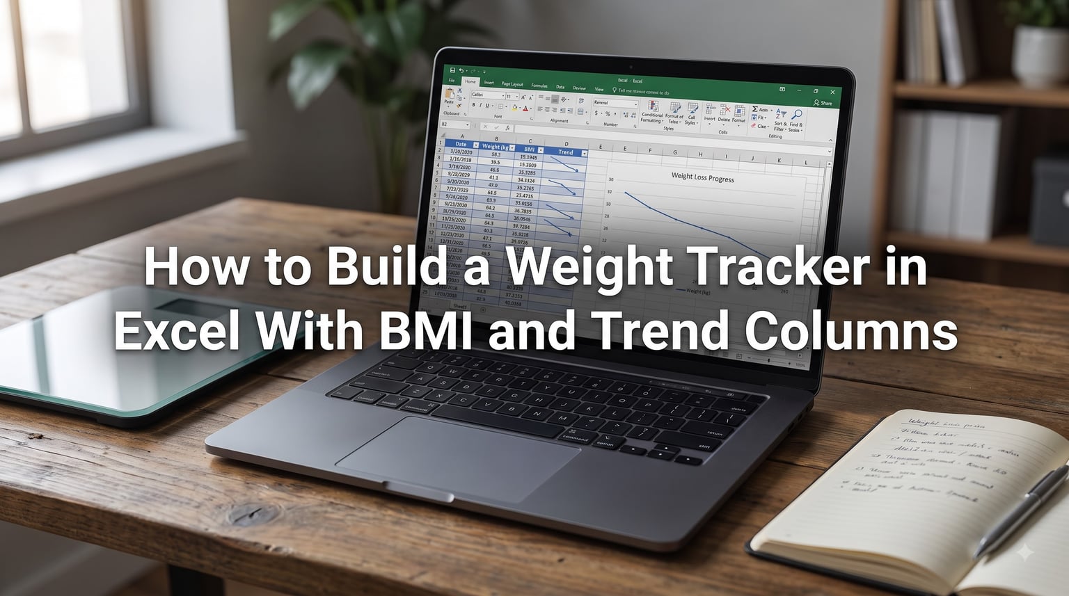
Tracking your weight in a spreadsheet gives you full control over your data, your formulas, and your privacy. Unlike subscription apps that lock your history behind a paywall, an Excel weight tracker lives on your computer and works the way you want it to. I have built dozens of these spreadsheets over the years for personal use, friends, and fitness challenges, and the same setup works every time.

In this guide, I will walk you through exactly how to build a weight tracker in Excel with BMI and trend columns from a blank workbook. You will learn the exact formulas for BMI, weekly weight change, cumulative loss, and percentage progress. I will also show you how to add a progress chart and a dashboard summary so your spreadsheet looks polished and stays motivating.

This tutorial works in Excel 2016 or later, including Microsoft 365 on Windows and Mac. Most steps also work in Google Sheets with minor formula adjustments. No macros, no add-ins, no coding required.

Table of Contents

• What You Need Before You Start
• How to Build a Weight Tracker in Excel With BMI and Trend Columns: Step-by-Step
• Step 1: Set Up Your Weight Tracker Columns
• Step 2: Add Weekly Weight Change Column
• Step 3: Add Cumulative Weight Loss Column
• Step 4: Create the BMI Calculation Column
• Step 5: Build a Progress Chart With Trend Line
• Step 6: Create a Dashboard Summary
• Advanced Tips for Your Weight Tracking Spreadsheet
• Tips for Accurate Weight Tracking
• Frequently Asked Questions
  • How can I create a weight tracker in Excel?
  • How to create a BMI calculator in Excel?
  • How to create a dynamic tracker in Excel?
  • How do I calculate weekly weight loss in Excel?
  • Can I track weight in stone and pounds in Excel?
• Start Tracking Your Progress Today

What You Need Before You Start

Before opening Excel, gather three pieces of information: your current weight, your height, and your target weight. You also need to decide whether you are tracking in pounds or kilograms, since the BMI formula changes depending on the unit.

I recommend starting with at least four weeks of past weigh-in data if you have it. This lets you see your trend columns and chart populate immediately instead of staring at a single row. If you do not have past data, just start fresh and the spreadsheet will grow week by week.

One key decision: pick a unit system and stick with it. Mixing pounds and kilograms in the same column will break your BMI formula and skew your trend calculations. I cover both unit systems below so you can choose the one that fits your scale at home.

How to Build a Weight Tracker in Excel With BMI and Trend Columns: Step-by-Step

Follow these six steps in order and you will have a fully functional weight tracking spreadsheet in about 20 minutes. Each step builds on the previous one, so do not skip ahead.

Here is what we are creating: a single worksheet with columns for Date, Weight, Target Weight, Weekly Change, Cumulative Change, Percentage Lost, and BMI. Below the data table, a line chart will visualize your progress against your goal.

Step 1: Set Up Your Weight Tracker Columns

Open a new blank workbook in Excel. In row 1, enter these column headers starting in cell A1:

A1: Date
B1: Weight
C1: Target Weight
D1: Weekly Change
E1: Cumulative Change
F1: Percent Lost
G1: BMI

Type your height in cell J1 and label it clearly in cell I1. For example, type “Height” in I1 and your height in inches in J1 (if using imperial) or in meters in J1 (if using metric). We will reference this cell in the BMI formula later.

Now enter your first row of data. In A2, type the date of your first weigh-in. In B2, type your starting weight. In C2, type your target weight. Leave columns D through G empty for now, since those are formula columns we will fill in the next steps.

Next, convert your data range into an official Excel Table. Select cells A1 through G2, then press Ctrl+T (or Cmd+T on Mac). Make sure “My table has headers” is checked, then click OK. Excel will name it Table1 by default and apply alternating row colors automatically.

The reason this matters: when you add a new row of data at the bottom of a Table, Excel copies your formulas down automatically. You never have to drag-fill again. This solves one of the most common frustrations people mention on Excel forums, where their tracker breaks because formulas were not extended to new rows.

Add a second row of data for the following week so you have two entries to work with. Enter the date in A3, your new weight in B3, and the same target weight in C3.

Step 2: Add Weekly Weight Change Column

The Weekly Change column shows how much your weight shifted compared to the previous entry. This is your most basic trend column and the one people check first each week.

In cell D3 (the second data row), enter this formula:

=[@Weight]-[@[Weight]] using structured references, or more practically: =B3-B2

This subtracts last week’s weight from this week’s weight. If you lost 2 pounds, the result will be negative 2. If you gained, it will be positive. I prefer keeping losses as negative numbers because it feels intuitive, but you can reverse the formula to =B2-B3 if you want losses to show as positive.

Since you are working inside an Excel Table, the formula will auto-fill down every new row you add. You do not need to copy it manually.

The first row (row 2) has no previous week to compare against, so leave D2 blank or enter a dash. If you want to avoid any confusion, wrap the formula in IFERROR to handle edge cases cleanly:

=IFERROR(B3-B2,"")

This displays nothing if there is no previous value instead of showing a zero or error. It keeps your spreadsheet clean.

Step 3: Add Cumulative Weight Loss Column

The Cumulative Change column tracks your total progress from your very first weigh-in. Unlike the weekly column that resets each entry, this one compounds over time so you can see the big picture.

In cell E2, enter this formula to anchor it to your starting weight:

=B2-$B$2

The dollar signs in $B$2 lock the reference to your starting weight cell. When Excel fills this formula down the column, every row will subtract that same starting value from the current weight. If you started at 200 pounds and now weigh 188, the cumulative column will show negative 12.

For the Percentage Lost column, enter this formula in cell F2:

=(B2-$B$2)/$B$2

Format this column as a percentage by selecting the column, right-clicking, choosing Format Cells, and selecting Percentage. Now you will see values like negative 6.0 percent instead of negative 0.06. This column is incredibly motivating because it translates raw numbers into meaningful progress.

If you are tracking weight gain rather than loss, these same formulas work perfectly. The numbers will simply be positive instead of negative, showing how much you have gained from your starting point.

Step 4: Create the BMI Calculation Column

BMI (Body Mass Index) is a standard screening tool that uses your height and weight to estimate whether you fall in a healthy range. Adding it to your weight tracker gives you context beyond raw pounds or kilograms.

If you are using metric units (kilograms and meters), the BMI formula in cell G2 is straightforward:

=B2/($J$1^2)

This divides your weight in kilograms by your height in meters squared. The $J$1 reference points to the height cell you set up in Step 1. The dollar signs lock it so every row uses the same height value.

If you are using imperial units (pounds and inches), the formula needs a conversion factor of 703:

=(B2/($J$1^2))*703

This converts the metric BMI formula to work with pounds and inches. Enter your height in inches in cell J1. For example, if you are 5 foot 8, your height in inches is 68.

Format the BMI column to show one decimal place so values read as 24.5 instead of 24.5193. Select the column, right-click, choose Format Cells, select Number, and set decimal places to 1.

Now add conditional formatting to color-code your BMI results. Select the BMI column, go to Home > Conditional Formatting > Highlight Cells Rules, and set up these ranges:

Below 18.5: Underweight (blue fill)
18.5 to 24.9: Normal (green fill)
25.0 to 29.9: Overweight (yellow fill)
30.0 and above: Obese (red fill)

To do this precisely, use Conditional Formatting > New Rule > Format only cells that contain. Create four separate rules for each range. The color coding gives you instant visual feedback every time you enter a new weight.

Step 5: Build a Progress Chart With Trend Line

A chart is what turns your weight tracking spreadsheet from a data dump into a motivational tool. I have seen people check their chart every single morning because watching the line drop is genuinely exciting.

Select your Date column (column A) and your Weight column (column B). Hold Ctrl while selecting so you grab both columns without the ones in between. Then go to Insert > Charts > Line Chart and choose the basic line option.

Excel will create a line chart showing your weight over time. But to make it truly useful, we need to add your target weight as a second line so you can see the gap between where you are and where you want to be.

Right-click the chart and choose Select Data. Under Legend Entries, click Add. Set the Series Name to “Target” and the Series Values to your Target Weight column (C2 through your last row). Now you will see two lines: your actual weight and your target.

For the trend line, click your weight line in the chart, right-click, and choose Add Trendline. Select Linear if your weight loss is steady, or Polynomial if your progress has ups and downs. The trend line smooths out daily fluctuations to show your overall direction.

Format the chart for maximum motivation. Right-click the target weight line and make it a dashed red line so it stands out. Make your actual weight line solid blue with markers at each data point. Add a chart title like “Weight Loss Progress” and axis labels for Date and Weight.

Resize the chart and place it below your data table or on a separate chart area to the right. As you add new weekly entries, the chart updates automatically since it references an Excel Table.

Step 6: Create a Dashboard Summary

A dashboard pulls your key numbers into one clean view so you do not have to scroll through rows of data. I like to place the dashboard at the top of the sheet or in cells to the right of the chart.

Create labeled cells for these summary stats:

Current Weight: =LOOKUP(2,1/(B:B""),B:B) (finds the last weight entry)
Starting Weight: =B2 (your first entry)
Total Lost: =B2-LOOKUP(2,1/(B:B""),B:B)
Current BMI: =LOOKUP(2,1/(G:G""),G:G)
Remaining to Goal: =LOOKUP(2,1/(B:B""),B:B)-C2

The LOOKUP formula might look intimidating, but it simply finds the last non-empty cell in a column. This means your dashboard always shows your most recent entry no matter how many weeks of data you accumulate.

For a cleaner approach, define named ranges for key cells. Go to Formulas > Name Manager > New. Create names like “StartWeight” pointing to B2, “TargetWeight” pointing to C2, and “Height” pointing to J1. Then your formulas read as =StartWeight-CurrentWeight instead of cell references. Named ranges make your spreadsheet easier to understand months later when you have forgotten what B2 meant.

Format your dashboard cells with large bold fonts and distinct background colors so they stand out. This is the area you will glance at every week, so make it visually appealing.

Advanced Tips for Your Weight Tracking Spreadsheet

Once your basic tracker is working, these enhancements take it to the next level. None of them are required, but each one solves a real problem that comes up in long-term tracking.

Add data validation. Prevent accidental text entries in your Weight column by selecting the column, going to Data > Data Validation, and allowing only decimal numbers between 50 and 500 (or whatever range fits your situation). This catches typos like entering 1800 instead of 180.

Use sparklines for mini-trends. Select the cell next to each row of data, go to Insert > Sparklines > Line, and select that row’s weight range. This creates a tiny inline chart that shows the micro-trend for each period. Sparklines are perfect for seeing momentum at a glance without taking up chart space.

Add a goal projection column. If you want to project when you will hit your target, create a column that divides your remaining weight to lose by your average weekly loss. The formula: =(B2-TargetWeight)/AVERAGE(D:D) estimates weeks remaining at your current pace.

Track in stone and pounds. If you are in the UK, create two input columns: one for stone and one for pounds. Then create a calculated column that converts to total pounds with =stone_cell*14+pounds_cell. Use the total pounds column for your BMI and trend calculations. This gives you familiar input units while keeping the math clean.

Add conditional formatting on the Weekly Change column. Set green fill for negative values (weight loss) and red fill for positive values (weight gain). This gives you instant color feedback every time you enter a new weight without having to read the numbers.

Tips for Accurate Weight Tracking

Your spreadsheet is only as good as the data you feed it. After years of tracking and reading hundreds of forum posts, here are the practices that produce reliable, meaningful data.

Weigh yourself at the same time of day, ideally first thing in the morning after using the bathroom and before eating or drinking. Your weight fluctuates 3 to 5 pounds throughout the day based on hydration, food, and activity. Consistent timing eliminates these variables.

Use the same scale every time. Different scales can differ by several pounds, and switching between them introduces noise into your trend data. If you must switch scales, note the date in your spreadsheet so you understand any sudden shifts.

Consider weekly weigh-ins rather than daily. Daily fluctuations can be discouraging and may not reflect real progress. A weekly entry on the same day each week smooths out water weight swings and gives your trend columns cleaner data to work with.

Use the Excel date shortcut Ctrl+; (Cmd+; on Mac) to insert today’s date instantly in the Date column. This saves time and prevents date formatting errors that happen when typing dates manually.

Remember that BMI is a screening tool, not a diagnostic. It does not distinguish between muscle and fat, so very muscular individuals may register as overweight despite being lean. Use BMI as one data point alongside how you feel, how clothes fit, and other measurements.

Frequently Asked Questions

Start Tracking Your Progress Today

You now have everything you need to build a weight tracker in Excel with BMI and trend columns. The setup takes about 20 minutes, requires no macros or add-ins, and gives you a spreadsheet that grows with you week after week. Your formulas will calculate automatically, your chart will update on its own, and your dashboard will always show your latest numbers.

The hardest part of any fitness journey is starting. Open Excel, follow the six steps above, and enter your first weigh-in today. A few months from now, you will have a complete dataset showing exactly how far you have come.

Disclaimer: This guide is for informational purposes only and is not medical advice. Consult your doctor before starting any weight loss program, especially if you have underlying health conditions.